7.6 Parameter Estimation of ERGM

7.6.1 Current Methods for ERGM

1. Approximation-based Algorithm:
   MCMC 샘플들로 likelihood function 을 최대화. typically used in finding MLE.
   • Maximum Pseudo-likelihood Estimation (MPLE, 1974).
   • Markov Chain Monte Carlo Maximum Likelihood Estimation (MCMCMLE, 1994).
   • Markov Chain Monte Carlo Stochastic Approximation (MCMCSA, 2002).
     • 이 위까지로는 model degeneracy issue 를 해결하지 못했음. 아래의 VTSAMCMC 가서야 해결함.
   • Varying Truncation Stochastic Approximation MCMC Method with Trajectory Averaging (VTSAMCMC, 2013).
2. Auxiliary Variable Markov Chain Monte Carlo (MCMC) Algorithm:
   normalizing constant 를 근사하거나, normalizing constant ratio \(\frac{\kappa(\theta)} {\kappa(\theta')}\) 를 cancel 하기 위해 auxiliary variable 들을 도입 (introduce). 베이지안 추론을 위해 사용. Bayesian inference.
   • The Exchange Algorithm.
   • Auxiliary Variable Metropolis-Hasting Algorithm (AVMH).
   • Adaptive Exchange Monte Carlo Algorithm (AEXMC).

7.6.2 Approximation-based Algorithm

7.6.2.1 Maximum Pseudo Likelihood Estimation (MPLE)

\(A\) 내부의 성분 간의 의존성 (high-order dependence wihin network) 을 무시한 채로, conditional independence 를 가정하여 조건부 likelihood 함수들의 series를 곱하는 것으로 pseudo-likelihood 함수를 근사함. ERGMS 의 조건부이며 pseudo-likelihood 는 아래와 같음. 이렇게 근사한 pseudo-likelihood 로 maximum likelihood estimator 를 approximate. 물론 이건 어디까지나 가장 간단한 방법으로서 제시되었을 뿐이고, 이 방법론은 의존성 구조를 완전히 무시했기 때문에 퍼포먼스가 구림.

\[ \begin{align} &logit \Bigg \{ P_\theta \Big (X_{ij} = 1 \Big | X_{ij}^c = x_{ij}^c \Big ) \Bigg \} &&= \theta ' g(x_{ij}^c) \\ \iff &\log PL(\theta, x) &&= \sum_{ij} \theta ' g(x_{ij}^c) \cdot x_{ij} - \sum_{ij}\log \left \{ 1+ \theta ' g(x_{ij}^c) \right \} \end{align} \]

\[ \begin{align} &logit \Bigg \{ P_\theta \Big (X_{ij} = 1 \Big | y_{ij}^c \Big ) \Bigg \} &&= \underbrace{\sum_{i=1}^P \theta_i ' S_i(y_{ij}^c)}_{\text{log of unnormalized density with \(y_{ij}^c\)}} \\ \iff &\log PL(\theta, y) &&= \underbrace{\sum_{ij} \theta ' S(y_{ij}^c) \cdot y_{ij} - \sum_{ij}\log \left \{ 1+ \theta ' S(y_{ij}^c) \right \}}_{\text{not a proper likelihood}} \end{align} \]

• advantage: simple one / don’t need to generate auxiliary networks
• disadvantage: parameter estimates is not good because MPLE ignores high-order depedence

7.6.2.2 MCMC MLE

1. with initial guess of parameter -> generate auxiliary networks
2. with auxiliary networks -> update parameter estimates

패러미터 \(\theta^{(0)}\) 에 대해 이하와 같은 initial guess 가진다고 하자.

\[ l(\theta) = \theta ' S(y) - \log k(\theta)\\ l(\theta^{(0)}) = \theta^{(0)} ' S(y) - \log k(\theta^{(0)}) \]

\[ l(\theta)-l(\theta^{(0)})=(\theta-\theta^{(0)})^{t}S(y)-\log \frac{\kappa(\theta)}{\kappa(\theta^{(0)}} \]

distribution \(f(x|\theta^{(0)})\) 에서 생산된 MC 샘플들로부터 \(\kappa(θ)\) 근사. 이때 \(\theta^{(0)}\) 는 \(\theta\) 의 initial 측정값. MCMC 시뮬레이션을 통해 \(f(x_{obs}|\theta^{(0)}\) 으로부터 랜덤샘플 \(x_1 , \cdots, x_m\) 을 draw. 이 경우 log-ratio likelihood 는 \(m \rightarrow \infty\) 에서 이하와 같이 근사 가능.

\[ I(\theta)-I(\theta^{(0)})=(\theta-\theta^{(0)})^{t}g(x_{\mathrm{obs}})-\log\left[\frac{1}{m}\sum_{i=1}^{m}\exp\left\{(\theta-\theta^{(0)})^{t}g(x_{i})\right\}\right] \]

따라서 \(\theta\) 를 경유해서 \(I(\theta)-I(\theta^{(0)})\) 를 극대화하는 작업을 통해 결국 \(\hat \theta_{MLE}\) 를 근사할 수 있게 된다.

MCMLE 의 퍼포먼스는 \(\theta^{(0)}\) 의 선택에 좌우된다. \(\theta^{(0)}\) 이 MLE 의 참값의 attraction region 에 존재하지 않는다면, 해당 방법론은 suboptimal 해로 수렴해버리거나, 최악으로는 converge 실패 가능성도 있음.

7.6.2.3 MCMC Stochastic Approximation

exponential family 에 대한 이론을 통해, 우리는 ERGMs을 maximize 하는 것은 \(E_{\hat \theta} \Big \{ g(X) \Big \} = g(x_{obs})\) 라는 system 을 푸는 것과 동일하다는 것을 알 수 있다. 이 system 의 성립 여부는 이하와 iff (\(\iff\)).

1. \(\hat \theta = \hat \theta_{MLE}\)
2. Independent network generation
3. Parameter estimation update with stochastic approximation

이 방법론은 independent 네트워크 샘플을 생산하는데에는 비효율적이다. 각 샘플 \(x_{k+1}\)을 생산하기 위해 요구되는 이터레이션 스텝의 갯수는 order of \(100 n^2\). 이때 \(n\)은 node 의 갯수.

7.6.3 Auxiliary Variable MCMC-based Approaches

7.6.3.1 Exchange Algorithm

normalizing constant ratio \(\frac{\kappa(\theta)}{\kappa(\theta')}\) 따위의 auxiliary 변수로 분포 \(f(x | \theta)\) 를 augment. 이는 시뮬레이션 중에 canceled.

1. 후보 point \(\theta ' \sim q(\theta ' | \theta, x)\) 를 생산
2. perfect sampler 사용해서 auxiliary 변수 \(y \sim f(y | \theta ')\) 를 생산
3. \(\theta'\)를 with probability \(1 \wedge r(\theta, \theta ' \Big | x)\)로 채택. 이때

\[ r(\theta, \theta ' \Big | x) = \frac{\pi(\theta')}{\pi(\theta)} \cdot \frac{f(x \Big | \theta ' )}{f(x \Big | \theta )} \cdot \frac{f(y \Big | \theta)}{f(y \Big | \theta')} \cdot \frac{q(\theta \Big | \theta ' , x)}{q(\theta ' \Big | \theta , x)} \]

exchange 알고리즘은 Ising 이나 autologistic 과 같은 일부 discrete 모델에는 잘 작동. 하지만 perfect sampling 이 적용되지 않는 많은 다른 모델에는 적용할 수 없다. 우리는 MCMC 샘플을 통해 auxiliary 변수 \(y\)를 생산할 수 있지만, 수렴 문제 부분에서 이론적인 흠결이 있음. 만약 MCMC 샘플의 mixing이 매우 느리다면 딴놈이 아니라 \(\theta_0\) 가 매우 높은 확률로 채택되어버림. 그리고 이 MCMC 샘플의 mixing 이 느린 것 자체가 ERGMs 의 일반적인 특징임. 이래서 문제.

7.6.3.2 Monte Carlo MH Algorithm

MH 알고리즘의 MC 버전. 각 이터레이션에서 MCMH 알고리즘은 unknown normalizing constant ratio \(\frac{\kappa(\theta)}{\kappa(\theta')}\) 를 MC estimate와 importance 샘플링 접근법으로 대체한다.

exchange 알고리즘과 다르게, MCMH 알고리즘은 perfect sampler 요구조건을 빗겨간다. 따라서 perfect sampler 를 못 쓰는 다수의 통계문제에 대해서도 얘를 쓸 수 있음. 하지만 얘도 여전히 수렴 문제가 존재함. 얘의 경우에는 importance sampling estimator 가 유한한 숫자의 샘플로는 ratio의 참값 \(\frac{\kappa(\theta)}{\kappa(\theta')}\) 에 수렴하지 못할 수도 있음.

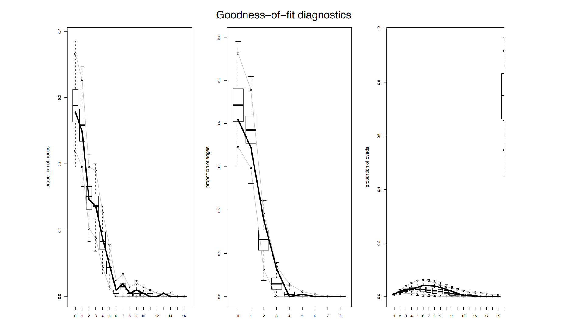
FIGURE 7.13: Goodness-of-fit Plots, for ERGMs - for the high school student friendship network

7.6.4 Varying Trunction Stochastic Approximation MCMC

ERGM 의 likelihood 함수는

\[ \begin{align} &f(y | \theta ) = \frac{1}{\kappa(\theta )} \exp \Big \{ \theta' S(y)\Big \}, &&\theta = (\theta_1 , \cdots, \theta_d)', &&S(y) = \Big( S_1 (y), \cdots, S_d(y) \Big)' \end{align} \]

이때 \(\kappa(θ)\)를 특정할 수 없다 (intractability)는 점과 모델 degeneracy 때문에, \(\theta\)를 정확하게 추정하는 것은 어렵다. 이 문제는 varying truncation stochastic approximation MCMC 를 사용하는 것으로 해결 가능.

Normalizing constant 는 \(\kappa(\theta) = \sum_{\text{all possible }y} \exp \Big \{ \theta ' S(y)\Big\}\).

이로 인해 촉발되는 문제는?

1. MPLE: dyadic 독립이 가정되어 있다. 이건 observed 네트워크가 무엇이냐에 대해 과하게 의존.
2. MCMLE: \(\theta^{(0)}\) 을 어떻게 고르느냐에 대해 과하게 의존. local 최적해로 수렴해버리거나 모델 degeneracy 로 수렴 자체가 실패하기도.

7.6.4.1 MCMC Stochastic Approximation

\(h(\theta) = 0\) 형의 system 을 풀자. 고전적인 SA 알고리즘은 이하와 같은 형태를 띈다. (\(a_k\) , \(h\), \(\omega_k\) 에 대한) 적절한 조건 하에서, 이 알고리즘은 해로 수렴한다는 것을 실제로 보이는 것이 가능하다.

$$ \[\begin{align} \theta_{k+1} &= \theta_k + a_k Y_k \\ &=\theta_k + a_k \Big \{ h(\theta_k) + \omega_k \Big \}, && k \ge 0 \end{align}\] $$

• \(Y = h(\theta) + \omega\) 는 noisy estimate
• \(\omega\) 는 mean-zero noise.

\(\theta_{MLE}\) 를 찾는 것은 exponential family 안에서 \(E_\theta \{ S(Y) \} = S(\mathbf y_{obs})\) 의 해를 찾는 것과 equivalent. 이는 이하의 단계를 거친다. 다만 이는 independent 네트워크 샘플을 생산하는데 있어 비효율적일 수밖에 없음. order of \(100n^2\) 이라 연산을 엄청 먹으니까.

1. \(\mathbf y^{k+1} \sim f(\mathbf y | \theta^{(k)}\)를 샘플링 (independence 네트워크 생산)

각 arc 변수 \(Y_{ij}\)가 독립적으로 정해지는 랜덤 그래프에서 시작. 이 변수에는 0 혹은 1이 0.5 확률로 할당. 이 랜덤 그래프를 Gibbs 샘플러든 MH 알고리즘이든 써서 업데이트.

2. SA 를 통해 패러미터 estimate \(\theta^{(k+1)} = \theta^{(k)} - a_k D^{-1} \Big \{ U( \mathbf y_{k+1}, \bar {\mathbf y}_{k+1} ) - \mathbf S (\mathbf y_{obs} ) \Big \}\) 절차 따라서 업데이트. where

$$ \[\begin{align} U( \mathbf y_{k+1}, \bar {\mathbf y}_{k+1} ) - \mathbf S (\mathbf y_{obs} ) \Big \} &= P(\bar {\mathbf y}_{k+1} \Big | \mathbf y_{k+1} ) \cdot \mathbf S (\mathbf {\bar y}_{k+1} ) \Big \{ 1-P(\mathbf {\bar y}_{k+1} \Big | \mathbf y_{k+1} ) \Big \} \cdot \mathbf S (\mathbf {\bar y}_{k+1} ) \\ \mathbf {\bar y}_{k+1} &= 1- \mathbf y_{k+1} \end{align}\] $$

7.6.4.1.1 Model Degeneracy

\(\theta\)을 어떻게 정하느냐에 따라 모델은 그것의 확률을 (Complete (fully connected) 거나 empty (entirely unconnected) 네트워크와 같은) 1개 혹은 소수의 그래프에만 한정시켜서 부어버릴 수도 있다. (탐색 효율 쓰레기됨) 이 문제를 해결하기 위해선 탐색 전에 degeneracy 리전을 거의 포함하지 않는 패러미터 스페이스를 가지는 모델로 특정할 필요가 있다. 근데 이게 진짜 드럽게 어려움.

7.6.4.2 Varying Truncation SAMCMC for ERGMs

알고리즘 proceeds 전 Setup: for some constants \(k_0>1\), \(\eta \in (\frac{1}{2},1)\), \(\xi \in (\frac{1}{2},\eta)\), \(C_a > 0\), \(C_b >0\), set as below.

$$ \[\begin{align} &a_k = C_a \left( \frac{k_0}{(k_0 \vee k)}\right)^\eta, &&b_k = C_b \left( \frac{k_0}{(k_0 \vee k)}\right)^\xi \tag{C_1} \end{align}\] $$

Next,

\[ \bigcup_{s \ge 0} \mathcal K_s = \Theta, \; \; \; \text{where } \mathcal K_s \subset \text{int}(\mathcal K_{s+1}) \tag{C_2} \]

And also,

• \(\mathcal X\): a space of social network
• \(\mathcal T\): \(\mathcal X \times \Theta \rightarrow \mathcal X_0 \times \mathcal K_0\) (reinitialization mechanism)
• \(\sigma_k\): 이터레이션 \(k\) 까지 수행되는 reinitialization 의 숫자. (\(\sigma_0 = 0\))

---

Proceeds:

1. Gibbs 샘플러 사용해 \(m\) sweeps 번 interate 해서 auxiliary network \(y_{k+1} \sim f(y | \theta^{(k)})\) 생산

2. Set \(\theta^{(k + \frac{1}{2})} = \theta^{(k)} + a_k \Big \{ S(y_{k+1}) - S(y_{obs}) \Big \}\)

3. Set

$$ \[\begin{cases} \sigma_{k+1} = \sigma_k \; \text{ and } \left( y_{k+1}, \theta^{(k + {1})} \right) = \left( y_{k+1}, \theta^{(k + \frac{1}{2})} \right) \; \; \; \; \; \; \; \; \; \; & \| \theta^{(k + \frac{1}{2})} - \theta^{(k)} \| \le b_k, \; \; \theta^{(k + \frac{1}{2})} \in \mathcal K_{\sigma_k} \\ \sigma_{k+1} = \sigma_k+1 \; \text{ and } \left( y_{k+1}, \theta^{(k + {1})} \right) = \mathcal T \left( y_{k}, \theta^{(k)} \right) & o.w. \end{cases}\]

$$

7.6.4.2.1 Trajectory averaging estimator

trajectory averaging estimator \(\bar \theta_n = \frac{1}{n}\sum_{k=1}^n \theta^{(k)}\) 에 의해 \(\theta\) 를 estimate 가능.

실전에서는 estimate 의 variation 을 줄이기 위해 대신 \(\theta\) estimate 에 \(\bar \theta (n_0 , n) = \frac{1}{n-n_0}\sum\limits_{k=n_0+1}^n \theta^{(k)}\) 을 자주 사용함. 이 때 \(n_0\) 는 burn-in 이터레이션의 숫자.

• Free parameters
  • Free parameters: \(\{a_k\}\), \(\{b_k\}\), \(\{\mathcal K_s, \; s \le 0\}\), \(m\)
  • \(k_0 = 100\), \(\eta = 0.65\), \(\xi = \frac{0.5 + \eta}{2}\).
  • \(C_a\), \(C_b\): adjusted for different examples
  • choose \(\mathcal K_0\) to be around MPLE.
  • 이 article 에선 \(\mathcal K_{s, 1} = \Big [ -4(s+1), 4(s+1) \Big]\), \(\mathcal K_{s, 2} = \cdots = \mathcal K_{s, d} = \Big [ -2(s+1), 2(s+1) \Big]\) 로 설정.
  • \(m=1\)

7.6.4.2.2 Numerical Examples

Methods: MCMLE, SAA (Stochastic Approximation Algorithm), Varying truncation SAMCMC SAMCMC: independent 5 runs(each of 200,000 iterations) (m=1, Ca = 0.01, Cb = 1000, η, ξ, κs are defalut)

?????????????????\?????????????????\?????????????????\?????????????????\?????????????????\?????????????????\?????????????????\?????????????????\?????????????????\?????????????????\?????????????????\?????????????????\?????????????????\?????????????????\?????????????????\?????????????????\?????????????????\?????????????????\?????????????????\?????????????????\?????????????????\?????????????????\?????????????????\?????????????????\?????????????????\?????????????????\?????????????????\?????????????????\?????????????????\?????????????????\?????????????????\?????????????????\?????????????????\?????????????????\?????????????????\?????????????????\?????????????????\?????????????????\

7.6.5 Conclusion

SAMCMC 알고리즘의 varying truncation 은 ERGM 에 적용 가능. 여기서는 estimator 가 degeneracy region 으로 향하는 걸 reinitialization 에 의해 방지. estimator 는 ERGM 의 MLE로 converge 하며, 이는 asymptotic 하게 \(N\) 을 따르며 asymptotic 하게 efficient. 이는 normalizing constant 를 감당하고서라도 model degeneracy problem 를 해결할 수 있다는 점에서 유용.